Folk wisdom claims 7 shuffles is sufficient to thoroughly mix up a deck of cards. This claim originates from a paper published in 1986 by David Aldous and Persi Diaconis and summarized in the New York Times in 1990.
Does my mediocre shuffling reflect this common wisdom? This post is an attempt to investigate that question.
Table of Contents
Collecting Data
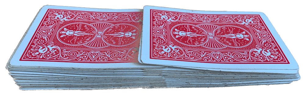
The first step to assessing my shuffling performance is to investigate a few real world shuffles. To start I recorded 5 the results of 5 shuffles by hand to get a sense of the variation in the distribution. Each run involved shuffling the deck with a riffle shuffle but not aligning the left and right hand piles:
The resulting order was then recorded as a string of 1s (card from left hand) and 2s (card from right hand). The 5 initial shuffles were:
1112212122121212121212121212121212121212121212111221
1222212212212121221212121212121212222112112211221122
2221121212211212112121221211221212121122222112212122
2222122121221121212121122112211222121222211222112211
2221221221122221212112221122121212212211122122121221
Eyeballing here shows quite a bit of variation from shuffle to shuffle. I set out to record the results of 100 independent shuffles to start to quantify the distribution.
Shuffling - Head On
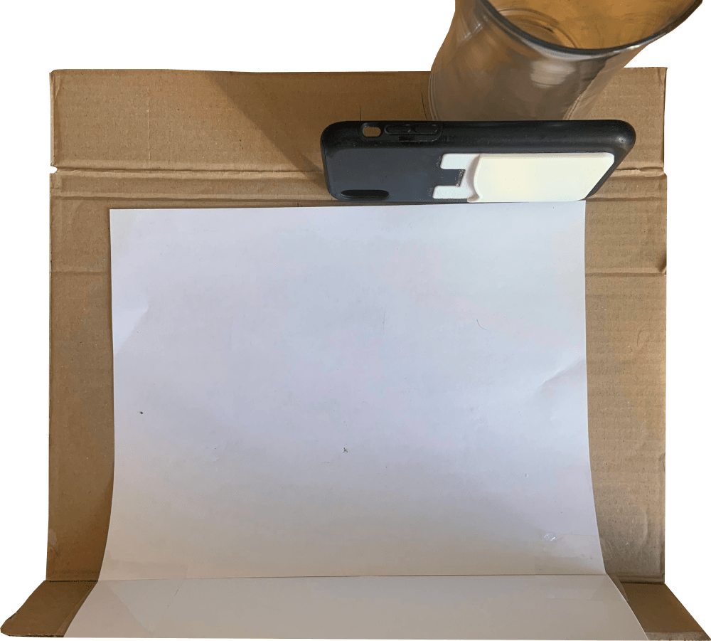
The most straightforward approach seemed to be recording the cards falling during the shuffling sequence in slow motion (phone camera can capture at 240fps). The video was recorded in a semi-reproducible environment to ease processing:
A sample of the resulting video looks like:
Even at 240fps some of the faster cards aren't captured in transit, and the ones that are captured are blurry and tough to detect with any sort of definable edge or feature. We can address this by instead capturing the face of the shuffle pile as it changes (the time constant between dropping new cards is much larger than the one associated with the drop itself).
Shuffling - Angled Down
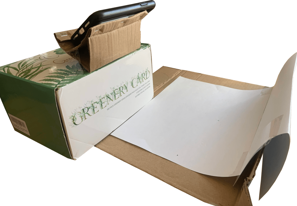
The new and improved data collection environment involved even more cardboard:
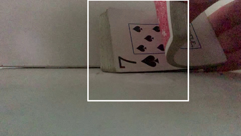
Initially, the video collected during a shuffle looks promising. It is easy to identify transitions between shuffled cards and which hand is dropping the card:
However, when we look a little closer we don't notice any funny business:
Which is a problem because there was indeed some funny business. The 3 of clubs was tucked between the 9 and 4 of spades.
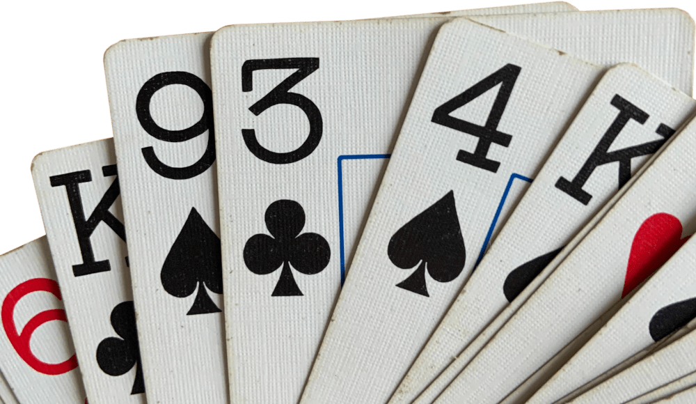
You can make out the edge of the card in the video, but we never see the face because the shuffle isn't perfect and I release both the 3 of clubs and the 4 of spades at the same time.
This doesn't happen in every shuffle, but it does happen occasionally. We might argue that we can just throw out shuffles where we don't process 52 different cards to avoid the missed card measurement error. However, that would introduce a systematic bias into the measurement - we would be removing all the worst shuffles from the dataset and our resulting impression of our shuffling performance would be better than it should be.
Post Shuffle Conveyor Belt
We had a lot of cardboard to spare and I had to try getting the power tools involved somehow. The gravity-fed rubber band and drill feeder worked, but was more trouble than it was worth.
Post Shuffle Riffle
One way to address the systematic bias mentioned above is to decouple the event of the shuffle from the recording of it. That way, if we were to make an error that invalidates the recording, we have no reason to expect the error would alter the perceived distribution. One way to do this is to record the order of the cards after the shuffle. If we record the order before and after each shuffle we can back out the 1s and 2s that make up our riffle model.
If we take the cards and riffle them in front of the camera we can then look for cards in each frame and record the order.
This strategy is also prone to missing a card, but we can address the problem this time. We can record two different riffles and compare the resulting orders, using the knowledge from the second recording to fill in gaps or resolve discrepancies. If we are unable to order the cards with sufficient confidence we can drop that shuffle from the dataset without introducing bias.
Transfer Learning Post Processing
Of course, we won't be processing the video by hand. I was hoping to use this project to do some in-the-wild machine learning so we will leverage that here. There are a few projects on Github doing playing card detection but they are generally looking for whole cards on specific backdrops. We will train a new model and make use of the controlled environment it is being deployed in.
Data Labelling
We'll start off by labelling a bit of the data we collected to train on. We'll use Python and OpenCV to flip through the video files and write frames:
import cv2Most of the models we will be considering want small and square images as input. Fortunately, we riffled in a very consistent fashion so we can crop all the video frames in the same small square. We'll use 224x224 as our image size for now.
def prep_frame(f):
    return cv2.resize(f[0:800, 700:1500], (224,224))
We can then run through the video frame by frame and label each image. To make things easier we will consider two different classification problems for each frame independently - suit and rank.
To start with the suits we need to:
Read a new frame from a video
Crop the frame as dictated above
Show the frame and wait for a keypress
Upon keypress:
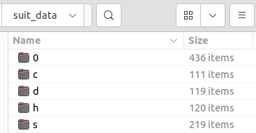
If "c", "s", "h", "d", or "0" (for clubs, spades, hearts, diamonds, none) save to that directory with unique ID generated from frame counter
If "q" then quit the program
If other key then skip the frame and go to the next
Repeat until the end of the video is reached
cap = cv2.VideoCapture("INPUT.MOV")

i = 0

while True:

    i+=1

    ret, f = cap.read()
    if not ret:
        print("End of video")
        break

    f = prep_frame(f)

    cv2.imshow('frame', f)
    key = cv2.waitKey(0)

    if chr(key) in 'cshd0':
        cv2.imwrite("suit_data/" + chr(key) + "/" + str(i) + ".jpg", f)
    elif chr(key) in 'q':
        break

cap.release()
cv2.destroyAllWindows()
After running through all the video frames we should have generated a bit of training data for each suit.
And we can verify the classifications look decent:
import matplotlib.pyplot as plt
from mpl_toolkits.axes_grid1 import ImageGrid
import numpy as np

fig = plt.figure(figsize=(10., 6.))
grid = ImageGrid(fig, 111, nrows_ncols=(3, 5), axes_pad=0.1, share_all=True)

grid[0].get_yaxis().set_ticks([])
grid[0].get_xaxis().set_ticks([])

grid[0].set_title("C")
grid[1].set_title("D")
grid[2].set_title("H")
grid[3].set_title("S")
grid[4].set_title("0")

ims = []
for _ in range(3):
    for s in "cdhs0":
        im_file = random.choice(os.listdir("suit_data/"+s))
        im = cv2.imread("suit_data/"+s+"/"+im_file)
        ims.append(im[...,::-1])

for ax, im in zip(grid, ims):
    ax.imshow(im)

plt.show()
Rinse and repeat for the ranks of each card.
Model Training
Now that we have a subset of our data labelled we can train an algorithm to label the rest of the videos we will take.
There are plenty of models out there that do a great job of parsing images and learning their requisite features. We would like to take a model that is good at understanding images and have it learn to classify our specific images. This is the definition of transfer learning.
We'll follow along with the TensorFlow example detailed here for the most part.
First bring in a few packages we will need:
import os

import matplotlib.pylab as plt
import numpy as np

import tensorflow as tf
import tensorflow_hub as hub
The we can browse through the available models on TensorFlow Hub for a suitable classification model. Our problem is pretty easy, and we will have no trouble using a small MobileNet model. This model takes in 224x224 images (which is what we saved our training data at, so no need to resize).
model_name = "mobilenet_v2_100_224"
model_handle = "https://tfhub.dev/google/imagenet/mobilenet_v2_100_224/feature_vector/5"
image_size = (224,224)
batch_size = 16
data_dir = "suit_data"
We'll use Keras as our framework. Keras provide a convenient API to split up our dataset:
def build_dataset(subset):
      return tf.keras.preprocessing.image_dataset_from_directory(
        data_dir,
        validation_split=.20,
        subset=subset,
        label_mode="categorical",
        seed=123,
        image_size=image_size,
        batch_size=1)
Which we can use to generate a training and a validation dataset:
train_ds    = build_dataset("training")
val_ds      = build_dataset("validation")
And record a few pieces of information before we change the datasets:
train_size  = train_ds.cardinality().numpy()
val_size    =   val_ds.cardinality().numpy()
class_names = tuple(train_ds.class_names)
We will want to pre-process our image inputs and introduce some artificial warping to flesh out the data set.
First, the MobileNet model expects inputs from 0 to 1 and our current images contain pixel values from 0 to 255. We can fix that with a normalization layer that scales the data by 1/255. We'll want to do this to both the training and the validation data.
Next, we can move the images around a bit to resemble changes we might see in new data. These changes could consist of:
rotation
vertical translation
horizontal translation
zoom
contrast
We will only want to apply these mutations to the training data.
normalization_layer = tf.keras.layers.Rescaling(1. / 255)

preprocessing_train = tf.keras.Sequential([
    normalization_layer,
    tf.keras.layers.RandomRotation(0.1),
    tf.keras.layers.RandomTranslation(0, 0.2),
    tf.keras.layers.RandomTranslation(0.2, 0),
    tf.keras.layers.RandomZoom(0.2, 0.2),
    tf.keras.layers.RandomContrast(0.1),
])

preprocessing_val = tf.keras.Sequential([
    normalization_layer
])
Then we can take our data, stick it into batches, and apply the preprocessing described above to get it all ready to go. Note - we need to add a repeat() call to our training data to ensure we can make enough data during the training runs (this seems weird to me?).
train_ds = train_ds.unbatch().batch(batch_size)
train_ds = train_ds.repeat()
train_ds = train_ds.map(lambda images, labels:(preprocessing_train(images), labels))

val_ds = val_ds.unbatch().batch(batch_size)
val_ds = val_ds.map(lambda images, labels:(preprocessing_val(images), labels))
With the data ready to go we can prepare the model we are going to train. We need to add a few things to the main MobileNet model specified earlier to link everything together.
First, we need to add an input layer that is compatible with our RGB image size (224x224x3).
That can feed into the MobileNet model which gets downloaded from TensorFlow Hub.
We probably also want to include some dropout to prevent overtraining. 20% is a standard value to start with.
Finally, we need a Dense layer that will act as the classifier for the 5 different classes we have: none, clubs, diamonds, hearts, and spades. We will include some L2 regularization in this Dense layer to keep the kernel weights in check.
model = tf.keras.Sequential([
    tf.keras.layers.InputLayer(input_shape=image_size + (3,)),
    hub.KerasLayer(model_handle, trainable=True),
    tf.keras.layers.Dropout(rate=0.2),
    tf.keras.layers.Dense(len(class_names),
                          kernel_regularizer=tf.keras.regularizers.l2(0.0001))
])
Next we need to define how we want to train the model. This is done with model.compile() and some definitions.
Optimizer: Stochastic Gradient Descent with a small learning rate should work just fine, but feel free to poke around
Loss Function: Categorical Crossentropy is recommended when there are two or more labels that are one-hot encoded
from_logits = True must be used when the outputs are not normalized (as is the case when we have not soft-maxed the outputs)
label_smoothing takes our one-hot encoded outputs and smooths out the confidence a bit. Instead of encoding a club as [0,1,0,0,0] we encode it as, say, [0.01,0.96,0.01,0.01,0.01]. This can help regularization a bit.
Metrics: We will just monitor accuracy here
model.compile(
    optimizer=tf.keras.optimizers.SGD(learning_rate=0.005),
    loss=tf.keras.losses.CategoricalCrossentropy(from_logits=True, label_smoothing=0.1),
    metrics=['accuracy'])
Now we are ready to hit go on the training. We will train the model for 10 standard epochs and see how we're doing. This might take a few minutes.
steps_per_epoch = train_size // batch_size
validation_steps = val_size // batch_size
hist = model.fit(
    train_ds,
    epochs=10,
    steps_per_epoch=steps_per_epoch,
    validation_data=val_ds,
    validation_steps=validation_steps).history
Epoch 1/10
45/45 [==============================] - 44s 908ms/step - loss: 1.1458 - accuracy: 0.5792 - val_loss: 0.9850 - val_accuracy: 0.6420
Epoch 2/10
45/45 [==============================] - 39s 884ms/step - loss: 0.7227 - accuracy: 0.8610 - val_loss: 0.6280 - val_accuracy: 0.9205
Epoch 3/10
45/45 [==============================] - 40s 879ms/step - loss: 0.5971 - accuracy: 0.9368 - val_loss: 0.4976 - val_accuracy: 0.9886
Epoch 4/10
45/45 [==============================] - 40s 878ms/step - loss: 0.5762 - accuracy: 0.9579 - val_loss: 0.5069 - val_accuracy: 0.9943
Epoch 5/10
45/45 [==============================] - 39s 875ms/step - loss: 0.5431 - accuracy: 0.9691 - val_loss: 0.4847 - val_accuracy: 0.9943
Epoch 6/10
45/45 [==============================] - 39s 877ms/step - loss: 0.5381 - accuracy: 0.9705 - val_loss: 0.4756 - val_accuracy: 1.0000
Epoch 7/10
45/45 [==============================] - 40s 878ms/step - loss: 0.5272 - accuracy: 0.9803 - val_loss: 0.4778 - val_accuracy: 0.9886
Epoch 8/10
45/45 [==============================] - 40s 879ms/step - loss: 0.5193 - accuracy: 0.9803 - val_loss: 0.4799 - val_accuracy: 0.9886
Epoch 9/10
45/45 [==============================] - 39s 878ms/step - loss: 0.5227 - accuracy: 0.9789 - val_loss: 0.4841 - val_accuracy: 0.9830
Epoch 10/10
45/45 [==============================] - 39s 873ms/step - loss: 0.5221 - accuracy: 0.9733 - val_loss: 0.4808 - val_accuracy: 0.9943Tough to beat that. We probably could have gotten away with only 5 epochs, but oh well.

Finally, we can save the trained model:
model.save("suit_predictor")Deploying the Model
Now we need to use our models to identify all the cards in a riffle as it goes by and back out the shuffled string of 1s and 2s.
We'll start by loading in our models and the classes the predictions represent:
ranks = ('0', '2', '3', '4', '5', '6', '7', '8', '9', 'a', 'j', 'k', 'q', 'z')
rank_model = tf.keras.models.load_model("rank_predictor")

suits = ('0', 'c', 'd', 'h', 's')
suit_model = tf.keras.models.load_model("suit_predictor")

image_size = (224, 224)
We also need to make sure we do the same preprocessing on new images that we did on previous ones. That means cropping, scaling, and normalizing:
def prep_frame(f):
    return cv2.resize(f[0:800, 700:1500], (224,224))

normalization_layer = tf.keras.layers.Rescaling(1. / 255)
preprocessing_model = tf.keras.Sequential([normalization_layer])
def prep_input(inp):
    f = prep_frame(inp)
    arr = np.array([f[...,::-1].astype(np.float32)])
    return preprocessing_model(arr)
It is also going to be helpful to label the images directly as we monitor some results. We will borrow the draw_text function from this stackoverflow answer:
def draw_text(img, text, font=cv2.FONT_HERSHEY_PLAIN, pos=(0, 0), font_scale=3, font_thickness=2, text_color=(0, 0, 0), text_color_bg=(255, 255, 255)):
    x, y = pos
    text_size, _ = cv2.getTextSize(text, font, font_scale, font_thickness)
    text_w, text_h = text_size
    cv2.rectangle(img, pos, (x + text_w, y + text_h), text_color_bg, -1)
    cv2.putText(img, text, (x, y + text_h + font_scale - 1), font, font_scale, text_color, font_thickness)
Now we can see how we did by making predictions on new video frames. To prevent spurious classifications we will only record a card if we ID it two frames in a row.
cap = cv2.VideoCapture("INPUT2.MOV")

last_card = ""
card_order = []
viz = True

while True:
    ret, frame = cap.read()
    if not ret:
        print("No frame")
        break

    inp = prep_input(frame)

    preds = suit_model.predict(inp)
    suit_pred = suits[np.argmax(preds)]

    preds = rank_model.predict(inp)
    rank_pred = ranks[np.argmax(preds)]

    if rank_pred!="z" and suit_pred!="0":
        card = rank_pred + suit_pred
        if card == last_card and (len(card_order)==0 or card_order[-1] != card):
            card_order.append(card)
        if card == last_card and viz:
            draw_text(frame, rank_pred + suit_pred, pos=(800, 500))
        last_card = card

    if viz:
        cv2.imshow('frame', frame)
        if cv2.waitKey(3) == ord('q'):
            break

cv2.destroyAllWindows()
If the video we processed above has two independent riffles in it we should end up with a card_order vector that is, ideally, 104 elements long with 52 unique elements. That probably won't be the case. Instead, we probably get something that looks like:
0d
8c
jc
0h
jh
9s
9d
kh
.
.
.
0s
9h
9d
as
0d
8c
jc
0h
jh
8s
9s
9d
kh
.
.
.
0s
9h
Our two most robust measurements should be the last card of the first riffle and the last card of the second riffle. We can use these to split the vector in half and start lining things up (we could also detect the break between riffle 1 and riffle 2 using the timestamps in the video). In the example above the last card would be the 9h.
After 9h split and align:

    9d
    as
    0d
0d  8c
8c  jc
jc  0h
0h  jh
jh  8s
9s  9s
9d  9d
kh  kh
.   .
.   .
.   .
0s  0s
9h  9h
Now we can crawl through the two vectors and look for similar neighbors. On the first pass we will just note what is missing and mark it with an empty character:
num_el = len(set(card_order))

last_card = card_order[-1]

r1 = card_order[:card_order.index(last_card)+1]
r2 = card_order[card_order.index(last_card)+1:]

i = 0
while i < num_el:
    if r1[i] == r2[i] or r1[i]=="  " or r2[i]=="  ":
        i += 1
        continue
    elif i > len(r1):
        r1.append("  ")
    elif i > len(r2):
        r2.append("  ")
    elif r1[i] == r2[i+1]:
        r1.insert(i,"  ")
    elif r2[i] == r1[i+1]:
        r2.insert(i,"  ")
    elif r1[i] == r2[i+2]:
        r1.insert(i,"  ")
    elif r2[i] == r1[i+2]:
        r2.insert(i,"  ")
    i = 0

[print(i,j) for i,j in zip(r1,r2)]
After alignment first pass:
9d
as
0d 0d
8c 8c
jc jc
0h 0h
jh jh
8s
9s 9s
9d 9d
kh kh
0s 0s
9h 9hThen we can crawl through again and determine what to do with the empty characters. We either toss them or infill based on how many other entries for that particular card we see elsewhere:
ord = []
for (e1,e2) in zip(r1, r2):
    if e1 == "  ":
        if card_order.count(e2) > 1:
            continue
        else:
            ord.append(e2)
    elif e2 == "  ":
        if card_order.count(e1) > 1:
            continue
        else:
            ord.append(e1)
    elif e1 == e2:
        ord.append(e1)
as
0d
8c
jc
0h
jh
8s
9s
9d
kh
0s
9hAlmost there. Our last step is to link two deck orders and back out the shuffle sequence. For example, we might see these two deck orders in a row:
as  8s
0d  as
8c  0d
jc  9s
0h  8c
jh  9d
8s  kh
9s  jc
9d  0h
kh  jh
0s  0s
9h  9h
To back out the order we first find where the cut happened and then iterate through the resulting deck to see which hand each card came out of:
def get_shuffle(o1, o2):
    i = 0
    for e in o2:
        if e==o1[i]:
            i+=1
        else:
            cut_loc = i
    lh = o1[:cut_loc]
    rh = o1[cut_loc:]

    o = ""
    il = 0
    ir = 0
    for e in o2:
        if il<len(lh) and e==lh[il]:
            o += "1"
            il += 1
        elif e==rh[ir]:
            o += "2"
            ir += 1
        else:
            ValueError("not feasible shuffle result")

    return o
o1 = ["as","0d","8c","jc","0h","jh","8s","9s","9d","kh","0s","9h"]
o2 = ["8s","as","0d","9s","8c","9d","kh","jc","0h","jh","0s","9h"]
get_shuffle(o1,o2)'211212211122'Whew. A lengthy process but the result is a decent data collection pipeline.
Building a Shuffling Model
A recording of 100 of my shuffles can be found here.
This part of the project is all done in Julia.
Data Exploration
Bring in a few packages
using Plots, StatsPlots
using Random
using Distributions
using StatsBase
using KernelDensity
using Trapz
And read in the data from the recorded file into a vector of vectors of Int.
S_rec = [[parse(Int,c) for c in l] for l in readlines("rec.txt")]One way we can "score" a shuffle is by counting the number of card runs there were. A perfect shuffle, with two piles of 26 cards interwoven one at a time, would score 52 on this metric.
function score_shuffle(S)
    score = 1
    for i in 2:52
        if S[i] != S[i-1]
            score += 1
        end
    end
    score
end
scores = score_shuffle.(S_rec)
plot(scores, st=:scatter, legend=false, smooth=true,
xlabel="Row", ylabel="Score")
Ooph. A large range of performance and definitely got tired over time. But is this any good? It is tough to evaluate without context. The Gilbert-Shannon-Reeds (GSR) model dates back to 1955 and is the de-facto distribution used to model a riffle shuffle. The model has two steps:
Split the deck into left and right piles ( and ) according to a binomial distribution
Drop the cards one at a time with probability
This can be implemented in Julia:
function gsr_shuffle()
    cut = rand(Binomial(52),1)[1]
    nl = cut
    nr = 52 - cut

    out = zeros(Int,52)
    for i in 1:52
        pl = nl / (nl + nr)
        if rand() < pl
            out[i] = 1
            nl -= 1
        else
            out[i] = 2
            nr -= 1
        end
    end

    out
end
Now we can make a bunch of GSR-shuffled decks and see how our scores compare.
S_scores = score_shuffle.(S_vec)

GSR_vec = [gsr_shuffle() for _ in 1:10000]
GSR_scores = score_shuffle.(GSR_vec)

histogram(scores,      label="Me",  bins=15:2:52, lw=2, alpha=0.5, norm=:probability)
histogram!(GSR_scores, label="GSR", bins=15:2:52, lw=2, alpha=0.5, norm=:probability,
    xlabel="Score", ylabel="Fraction")
Looks like we outperform the shuffling model by quite a bit on this metric! Our mean score turns out to be 33 vs 27 for the GSR shuffle. This indicates we should probably build our own model instead of assuming the GSR.
Building a Model
Deck Split
The first action in shuffling is splitting the deck into two halves. Ideally you end up with two stacks of 26 cards. The standard approach to modeling this action (the approach taken in the GSR model) is to draw the card split from a binomial distribution. Let's see if that looks decent for us.
split_vec = [count(s.==1) for s in S_vec]
histogram(split_vec, bins=16.5:1:35.5, xticks=17:35, normalize=:pdf, label="observed")
plot!(Binomial(52), st=:line, xlims=(17,35), label = "expected (binomial)",
    xlabel="Number of Cards in Left Hand", ylabel="Fraction of Cases")
The binomial distribution is not a great fit here. 84/100 cases I ended up with <26 cards in my left hand and the distribution is much sharper (centered around 24) than the binomial would indicate. We should fit a different distribution to this action.
Our distribution is discrete and univariate over the integers from (let's say) 16 to 36. We can come up with a few ways of generating the underlying distribution:
Use the measured histogram
Fit a known discrete distribution to the data
Fit a known continuous distribution to the data and round
Use the data to generate a kernel density estimator
Measured Histogram
The most straightforward way to translate our measurements into a discrete probability distribution is to assume the data directly describes the underlying distribution. This assumption is most likely to hold true when you have a lot of measured data that has borne out the entirety of the underlying distribution. This assumption may appear to be true when the measured histogram is smooth and well-shaped.
The data we have shows a 1% chance of drawing a 30, and a 0% chance of drawing a 29. This is a small discrepancy but seems unlikely to me to be true.
The resultant PMF would be identical to the histogram of measurements:

Known Discrete Distribution
The Distributions.jl package provides a collection of distributions and the ability to fit them to experimental data using (usually) maximum likelihood estimation. The distributions available for this functionality are shown below.
Binomial(52) - would result from drawing each card as either right or left with a fixed probability
Binomial(20) - would result from only randomly drawing the 20 middle cards with a fixed probability (and assuming the other 32 are split 16 left, 16 right)
Discrete Uniform - would result if every outcome in the possible solution space has the same probability
Geometric - usually interpreted as the number of trials needed for a single outcome to materialize. Tough to apply in this case.
Poisson - the probability of a given number of independent events occurring in a specific period of time. We don't expect card dropping events to be independent.
Among these distributions we expect the binomial (especially the binomial with a smaller number of chance draws) to perform the best. And indeed that is true, the Binomial(20) distribution (which resulted in a 39% chance that each of the 20 randomly drawn card ends up in my left hand) fits the data decently well as seen in the chart below.
One thing we might (definitely) want to do is truncate the distribution - we certainly don't ever want our split to be <0 or >52, and we probably wouldn't shuffle the cards if we had <16 or >36 cards in one hand, it just doesn't feel right. We'll apply 16-36 truncation in all the results going forward.
split_vec = [count(s.==1) for s in S_vec]
histogram(split_vec, bins=15.5:36.5, norm=:pdf, label="Measured", alpha=0.5)

f = fit_mle(Binomial, 52, split_vec)
f = truncated(f,16,36)
plot!(f, st=:line, label = "Binomial(52)", lw=2)

x = 16:36
f = fit_mle(Binomial, x[end]-x[1], split_vec.-x[1])
plot!(x, st=:line, pdf.(f, x.-x[1]), label = "Binomial(20)", lw=2)

distributions = [
    (DiscreteUniform,   "DiscreteUniform")
    (Geometric,         "Geometric")
    (Poisson,           "Poisson")
]
for d in distributions
    f = fit_mle(d[1], split_vec)
    f = truncated(f,16,36)
    plot!(f, st=:line, marker=false, label = d[2], lw=2)
end
plot!(xlabel="Number of Cards in Left Hand", ylabel="Fraction of Cases", xlims=(16,36), xticks=16:36)
Note - discrete distributions are plotted here as continuous for ease of viewing.

Known Continuous Distribution
Similarly to the discrete options, Distributions.jl provides a host of continuous distributions that can be easily fit to our experimental data.
distributions = [
    (Exponential,       "Exponential")
    (LogNormal,         "LogNormal")
    (Normal,            "Normal")
    (Gamma,             "Gamma")
    (Laplace,           "Laplace")
    (Pareto,            "Pareto")
    (Poisson,           "Poisson")
    (Rayleigh,          "Rayleigh")
    (InverseGaussian,   "InverseGaussian")
    (Uniform,           "Uniform")
    (Weibull,           "Weibull")
]

histogram(split_vec, bins=15.5:36.5, norm=:pdf, label="observed", alpha=0.5)

for d in distributions
    f = fit_mle(d[1], split_vec)
    f = truncated(f,16,36)
    plot!(f, st=:line, label = d[2], lw=2)
end
plot!(xlabel="Number of Cards in Left Hand", ylabel="Fraction of Cases", xlims=(16,36), xticks=16:36)
We can discount quite a few of these right off the bat and then we are left with the LogNormal, Normal, Gamma, and InverseGaussian distributions.
Log Normal - usually the result of an event which is the product of multiple independent random variables
Normal - usually the result of an event which is the sum of multiple independent random variables
Gamma - can be used to model wait times - such as when will the nth event occur?
Inverse Gaussian - if a normal distribution describes possible values of a random walk process at a fixed time, the inverse gaussian describes the possible times at which we might see a specific value of a random walk process.
In order to round these to the proper domain we can integrate them over the rounding range of each integer. In the end these all look practically identical:
distributions = [
    (LogNormal,         "LogNormal")
    (Normal,            "Normal")
    (Gamma,             "Gamma")
    (InverseGaussian,   "InverseGaussian")
]

histogram(split_vec, bins=15.5:36.5, norm=:pdf, label="observed", alpha=0.5)


for d in distributions
    f = fit_mle(d[1], split_vec)
    f = truncated(f,16,36)

    #Integrate
    x_ep = 15.5:36.5
    x_cp = 16:36
    y_cp = [cdf(f, x_ep[i+1]) - cdf(f, x_ep[i]) for i in 1:length(x_ep)-1]

    plot!(x_cp, y_cp, st=:line, label = d[2], lw=2)
end
plot!(xlabel="Number of Cards in Left Hand", ylabel="Fraction of Cases", xlims=(16,36), xticks=16:36)
You might be able to make a case for any of these. They all can fit the data we have pretty well. If pressed I might argue the normal distribution makes the most sense here so that's what I'll assume going forward.
Kernel Density Estimate
The other option we have when generating a distribution here is to take the measured histogram and apply some smoothing via kernel density estimation. This is a great choice if we ever just want to make sure we are drawing from something very close to the measured data. That might be nice if the underlying mechanisms are poorly understood or too complex to attempt to model.
The Julia package KernelDensity.jl makes this process easy. The main parameter of interest is the kernel bandwidth we use to smooth with - larger values will smooth over spurious measurements at the expense of pulling down peaks. Smaller measurements won't do much smoothing work and may capture more fine structure than you would hope.
This is also a continuous estimator - so we need to integrate over the relevant region to get a probability mass function over the integers.
histogram(split_vec, bins=15.5:36.5, norm=:pdf, label="observed", alpha=0.5)

for bw = [0.2, 0.5, 1.0, 2.0]
    k = kde(split_vec, boundary=(26-10, 26+10), bandwidth=bw)

    x = 16:0.01:36
    y = pdf(k, x)

    x_ep = 15.5:36.5
    x_cp = 16:36
    y_cp = [trapz(x[(x.>x_ep[i]) .& (x.<x_ep[i+1])], y[(x.>x_ep[i]) .& (x.<x_ep[i+1])]) for i in 1:length(x_ep)-1]

    plot!(x_cp, y_cp, lw=2, label="BW = " * string(bw))
end

plot!(xlabel="Number of Cards in Left Hand", ylabel="Fraction of Cases", xlims=(16,36), xticks=16:36)
A bandwidth of 0.5 smooths over the spurious 29-30 bump while retaining most of the rest of the structure, it probably wins the eye test here.
Winning Distribution
We can compare the leading solutions from each of the previous 4 sections:

At this point it comes down to either our understanding of the underlying mechanism that is driving the distribution or aesthetic preference. Let me know if you come up with a good causal model. In the meantime, I'll use the normal distribution with a mean of 23.8 and a standard deviation of 1.8.
Dropping Cards
After splitting the deck in two we start to drop cards from either our left or right hand. The GSJ model predicts that this will happen probabilistically, with the probability of dropping from either the left or the right according solely to the fraction of remaining total cards that are currently in that hand. Is this a good model for us?
GSR Calibration
We can view GSR as making a prediction each time we are about to drop a card. We can then look at what actually happened, and see if things that were supposed to happen 25% of the time actually happened 25% of the time. This kind of analysis is commonly referred to as model calibration.
We don't have perfect point estimates here - so we need to bucket the probabalities. Anything within the blue squares below is considered likely "calibrated". For example, the bottom left point says that whenever the model predicted an event to happen between 0-10% of the time, it actually happened 0% of the time.
The points are sized roughly corresponding to how many predictions they represent. We notice that the model does a pretty good job overall - the only time it is off by more than 10% is the 10-20% bucket which is only comprised of 50 observations. Not bad.
probs = Float64[]
outcs = Bool[]
cards = Int[]
for S in S_vec
    for (i,s) in enumerate(S)
        nl = count(S[i:end].==1)
        nr = count(S[i:end].==2)
        prob = nl/(nl+nr)
        outc = (s == 1)
        push!(probs, prob)
        push!(outcs, outc)
        push!(cards, nl+nr)
    end
end

edges = 0:0.1:1.0
binC  = 0.05:0.1:0.95

h  = fit(Histogram, probs, edges)
binindices = StatsBase.binindex.(Ref(h), probs)

outF = Float64[]
dps  = Int[]
for i in 1:length(binC)
    idx = binindices .== i
    push!(outF, count(outcs[idx]) / count(idx))
    push!(dps, count(idx))
end

X = vcat([[x-0.05,x-0.05,x+0.05,x+0.05,x-0.05,NaN] for x in binC]...)
Y = vcat([[x-0.05,x+0.05,x+0.05,x-0.05,x-0.05,NaN] for x in binC]...)
plot(X, Y, fill=true, label="Perfectly Calibrated", aspect_ratio=1, size=(500,500),
    xlabel = "Predicted Probability",
    ylabel = "Observed Probability",
    xticks = edges, yticks=edges)

outF[dps.<10] .= 0
dps[dps.<10]  .= 0
binX = [mean(probs[binindices.==i]) for i in 1:length(dps)]
scatter!(binX, outF, markersize=log.(dps/maximum(dps)).+9, label="Actual", legend=:topleft, xlims=(-0.05,1.05), ylims=(-0.05,1.05))
Differences from GSR
What are some ways in which we might differ from the GSR model? Perhaps we systematically favor the right or left hand at certain times:
side_ev = [mean([s[i] for s in S_vec]) for i in 1:52] .- 1
plot(side_ev, label="observed", ylims=(0, 1), ylabel="← Left Hand                Right Hand →", xlabel="Card Number", lw=2)

GSR_side_ev = [mean([s[i] for s in GSR_vec]) for i in 1:52] .- 1
plot!(GSR_side_ev, label="GSR model", lw=2)
It looks like we do systematically favor the right hand at the beginning and end of the shuffle.
Of particular interest in shuffling efficiency is runs of cards, do we have more or longer runs than the GSR model would predict?
Investigating Performance
[IN WORK]
Ingredients
pngquant
Gimp
ffmpeg
jpegoptim
iPhone 11
cardboard
Bicycle playing cards
Python 3.9.7
OpenCV 4.5.4
Matplotlib 3.3.4
Numpy 1.19.5
Tensorflow 2.7.0
Tensorflow_hub 0.12.0
Julia 1.7.1