You know that game everyone plays when watching the Superbowl? Where you buy a square for a dollar and then if the two last digits of the score at the end of the quarter end up corresponding to your square you win some money?
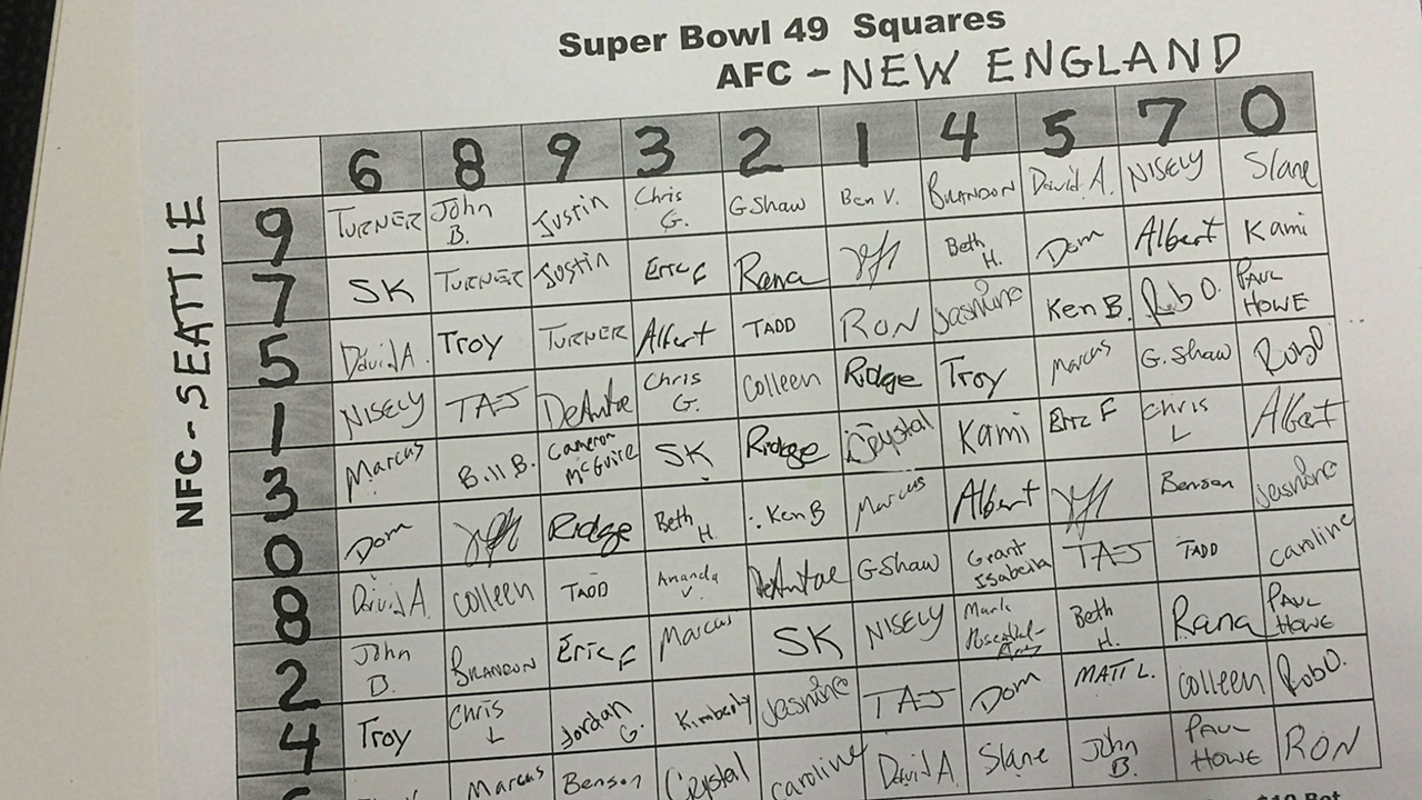
The numbers assigned to the rows and columns are typically randomly generated after all the squares are purchased, so the best squares like (0,0), (7,0) and (0,7), can't be knowingly purchased.
The random assignment prevents there from being any strategy involved with the selection of any one square. However, when purchasing multiple squares, you have the choice to buy your additional squares in a common row or column.
This project attempts to see what sort of statistical edge you might be able to glean from strategically purchasing multiple squares at your next Superbowl party.
Data
Model
Our ideal model determines, for both teams, the probability distribution over the following 5 possible outcomes:
ABCD - Different final digits for each quarter (e.g. 0,7,14,21)
AABC - 2 quarters share a final digit (e.g. 0,10,17,23)
AABB - 2 pairs of quarters share a final digit (e.g. 0,7,17,20)
AAAB - 3 quarters share a final digit (e.g. 7,10,17,17)
AAAA - All 4 quarters share a final digit (e.g. 0,10,10,20)
To simplify the problem we will use only the predicted final score as input to the model. This will cause us to miss any distinctive scoring characteristics (maybe this team never scores in the 3rd quarter) but we should capture the bulk of the predictive power. The best predictive data we will have should come from the Vegas betting line, which theoretically does all the modeling and predictive work for us. We will use the Over/Under and the spread to back out the implied point totals for both teams and use that as model inputs.
The historic data we will need to build the model thus looks something like (using the 2020 Superbowl as an example):
| GameID | Team | O/U | Spread | Q1 | Q2 | Q3 | End | Implied Total | ABCD | AABC | AABB | AAAB | AAAA |
|---|---|---|---|---|---|---|---|---|---|---|---|---|---|
| 202102070tam | tam | 54.5 | 3 | 7 | 21 | 31 | 31 | 25.75 | false | false | false | true | false |
| 202102070tam | kan | 54.5 | -3 | 3 | 6 | 9 | 9 | 28.75 | false | true | false | false | false |
Scraping
For some reason I could not find quarter-by-quarter scores of all historic NFL games as a tidy dataset anywhere. An excellent site https://www.pro-football-reference.com has all the desired information embedded in webpages that we can scrape.
Pro-football-reference has quarter-by-quarter scores available going back to 1920 and Vegas lines with a recorded spread and over/under going back to 1979. We will scrape all the games from 1979 to the present day.
In Julia webscraping can be done with the help of HTTP.jl, Gumbo.jl, and Cascadia.jl.
The scraping is performed in two passes, one to gather all the quarter scores and one to append all the Vegas lines.
To gather the quarter scores we follow this algorithm:
For each year in 1979-2020:
Find the weeks games were played from the Week Summaries buttons halfway down the page
For each week:
Read https://www.pro-football-reference.com/years/$YEAR/week_$WEEK.htm
Find all the "Final" Links for the displayed games
For each game:
Read https://www.pro-football-reference.com/boxscores/$GAMEID.htm
Find the first 3 quarter scores and the final score (ignore 4th quarter and overtime)
Write a line into the resulting .csv file for both teams
To append the Vegas lines to the table we follow this algorithm:
For each row in the data:
If the row is not yet populated with lines:
Read https://www.pro-football-reference.com/teams/$TEAM/$YEAR_lines.htm
Find all the rows in the "Vegas Lines" table
For each row:
Read the spread
Read the over/under
Find the matching gameID and TeamID in the data and record the spread and over/under
And then for final data preparation:
Sort by GameID
Make the quarter results cumulative
Remove the ~50 games where the over/under wasn't recorded
Calculate the implied points total for each row
One hot encode the quarter by quarter results into our 5 categories
Our resulting data has 20936 rows and looks like:
| year | week | id | team | opp | q1 | q2 | q3 | final | spread | OU | imp_tot | ABCD | AABC | AABB | AAAB | AAAA |
|---|---|---|---|---|---|---|---|---|---|---|---|---|---|---|---|---|
| 1979 | 1 | 197909010tam | det | tam | 0 | 7 | 7 | 16 | 3.0 | 30.0 | 13.5 | false | true | false | false | false |
| 1979 | 1 | 197909010tam | tam | det | 10 | 24 | 24 | 31 | -3.0 | 30.0 | 16.5 | false | true | false | false | false |
| 1979 | 1 | 197909020buf | mia | buf | 0 | 0 | 3 | 9 | -5.0 | 39.0 | 22.0 | false | true | false | false | false |
| 1979 | 1 | 197909020buf | buf | mia | 0 | 7 | 7 | 7 | 5.0 | 39.0 | 17.0 | false | false | false | true | false |
| 1979 | 1 | 197909020chi | gnb | chi | 0 | 0 | 3 | 3 | 3.0 | 31.0 | 14.0 | false | false | true | false | false |
| 1979 | 1 | 197909020chi | chi | gnb | 0 | 6 | 6 | 6 | -3.0 | 31.0 | 17.0 | false | false | false | true | false |
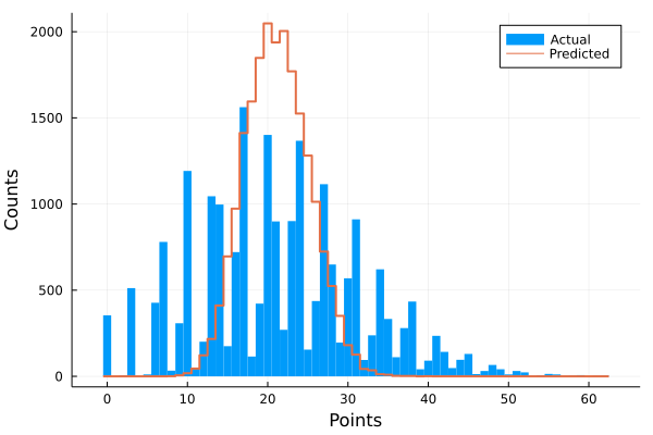
There is some interesting visualization we can do here. The actual total score and the predicted total score share the same median value (21) but the actual distribution has for more variance and is clumped around typical football scores.
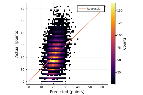
Turns out the betting lines are pretty good; the linear regression between the predicted and the actual score has a slope of 0.97 and an intercept <1.0.
What we really care about is how well the predicted score identifies the correct category.
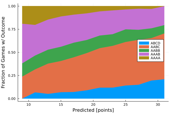
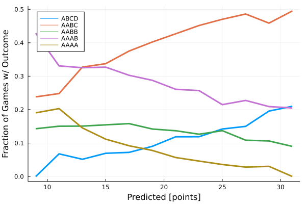
The results are impressively smooth and continuous. They generally follow some naive expectations: as the predicted score gets higher it becomes more and more likely that we end in higher variance outcomes, like ABCD or AABC, and less likely that we end in lower variance outcomes like AAAA.
Applied to the 2020 Superbowl, we can read out:
| team | spread | OU | imp_tot | P(ABCD) | P(AABC) | P(AABB) | P(AAAB) | P(AAAA) |
|---|---|---|---|---|---|---|---|---|
| tam | 3.0 | 54.5 | 25.75 | 0.14 | 0.48 | 0.13 | 0.22 | 0.03 |
| kan | -3.0 | 54.5 | 28.75 | 0.19 | 0.46 | 0.11 | 0.21 | 0.03 |
We now have a model that takes in the Vegas lines and returns the probability distribution across the 5 outcomes that we care about for square picking. Let's see what we can do with it!
Simulation
In Julia we can write a simple Monte Carlo simulation to play out many versions of the big game and see how well our bets score.
Each outcome will return 4 1-10 coordinates corresponsing to the row/column for each quarter.
using StatsBase

function ABCD()
    x = sample(1:10, 4, replace=false)
    return [x[1],x[2],x[3],x[4]]
end

function AABC()
    x = sample(1:10, 3, replace=false)
    return [x[1],x[1],x[2],x[3]]
end

function AABB()
    x = sample(1:10, 2, replace=false)
    return [x[1],x[1],x[2],x[2]]
end

function AAAB()
    x = sample(1:10, 2, replace=false)
    return [x[1],x[1],x[1],x[2]]
end

function AAAA()
    x = sample(1:10, 1, replace=false)
    return [x[1],x[1],x[1],x[1]]
end
We will roll against the probability distribution to see which outcome is randomly selected.
function get_outcome(P)
    roll = rand()
    if roll < P[1]
        return ABCD()
    elseif roll < P[1] + P[2]
        return AABC()
    elseif roll < P[1] + P[2] + P[3]
        return AABB()
    elseif roll < P[1] + P[2] + P[3] + P[4]
        return AAAB()
    else
        return AAAA()
    end
end
And the simulation will be run by comparing the random results to a vector of input coordinates. We can use multiple threads to speed things up.
function sim(coords, P1, P2; N=10000000)
    Y = zeros(Int16, N)
    payoff = 25

    Threads.@threads for i = 1:N

        t1 = get_outcome(P1)
        t2 = get_outcome(P2)

        for j=1:4
            for c in coords
                if t1[j]==c[1] && t2[j]==c[2]
                    Y[i] += payoff
                    break
                end
            end
        end

    end

    ȳ = sum(Y)/N
    s_y = sqrt(1/(N-1)*sum((Y.-ȳ).^2))
    ci_3σ = 3*s_y/sqrt(N)

    println()
    println("After $N runs:")
    println("Expected return on \$$(length(coords)) = \$$ȳ  (99% CI: \$$(round(ȳ-ci_3σ,digits=4)) - \$$(round(ȳ+ci_3σ,digits=4)))")
    println()

    return ȳ/length(coords)
end
With 1 Square
We can simulate the results with a single square to verify the expected return is neutral:
P1 = [0.14, 0.48, 0.13, 0.22, 0.03]
P2 = [0.19, 0.46, 0.11, 0.21, 0.03]
C = [(4,8)]
sim(C, P1, P2)
After 1000000 runs:
Expected return on $1 = $0.9989 (99% CI: $0.9813 - $1.0165)With 2 Squares
Two purchased squares can be aligned in 3 distinct ways:
✅✅ ✅⬜ ✅⬜
⬜⬜ ✅⬜ ⬜✅
P1 = [0.14, 0.48, 0.13, 0.22, 0.03]
P2 = [0.19, 0.46, 0.11, 0.21, 0.03]
C = [   [(1,1), (1,2)],
        [(1,1), (2,1)],
        [(1,1), (2,2)]
    ]
[sim(c, P1, P2) for c in C]
Expected return on $2 = $1.995625 (99% CI: $1.9707 - $2.0205)
Expected return on $2 = $2.001975 (99% CI: $1.9771 - $2.0269)
Expected return on $2 = $1.993350 (99% CI: $1.9686 - $2.0181)Hmm, no meaningful variation across those runs.
With 3 Squares
Three purchased squares can be aligned in 6 distinct ways:
✅✅✅ ✅✅⬜ ✅✅⬜ ✅⬜⬜ ✅⬜⬜ ✅⬜⬜
⬜⬜⬜ ⬜⬜✅ ✅⬜⬜ ✅⬜⬜ ✅⬜⬜ ⬜✅⬜
⬜⬜⬜ ⬜⬜⬜ ⬜⬜⬜ ⬜✅⬜ ✅⬜⬜ ⬜⬜✅
P1 = [0.14, 0.48, 0.13, 0.22, 0.03]
P2 = [0.19, 0.46, 0.11, 0.21, 0.03]
C = [   [(1,1), (1,2), (1,3)],
        [(1,1), (1,2), (2,3)],
        [(1,1), (1,2), (2,1)],
        [(1,1), (2,1), (3,2)],
        [(1,1), (2,1), (3,1)],
        [(1,1), (2,2), (3,3)],
    ]
[sim(c, P1, P2) for c in C]
Expected return on $3 = $2.981750 (99% CI: $2.9513 - $3.0122)
Expected return on $3 = $3.009350 (99% CI: $2.9790 - $3.0397)
Expected return on $3 = $2.999225 (99% CI: $2.9688 - $3.0296)
Expected return on $3 = $3.000825 (99% CI: $2.9705 - $3.0311)
Expected return on $3 = $3.008625 (99% CI: $2.9781 - $3.0392)
Expected return on $3 = $2.995750 (99% CI: $2.9656 - $3.0259)Still no variation in the results!
Exotic Probabilities
Perhaps we are only seeing neutral results because of the probability distribution we are using. Let's see if some more exotic probability distributions change things up.
With all outcomes equally likely:
P1 = [0.2, 0.2, 0.2, 0.2, 0.2]
P2 = [0.2, 0.2, 0.2, 0.2, 0.2]
C = [   [(1,1), (1,2), (1,3)],
        [(1,1), (1,2), (2,3)],
        [(1,1), (1,2), (2,1)],
        [(1,1), (2,1), (3,2)],
        [(1,1), (2,1), (3,1)],
        [(1,1), (2,2), (3,3)],
    ]
[sim(c, P1, P2) for c in C]
Expected return on $3 = $3.007775 (99% CI: $2.9747 - $3.0408)
Expected return on $3 = $2.992625 (99% CI: $2.9604 - $3.0248)
Expected return on $3 = $3.000900 (99% CI: $2.9683 - $3.0335)
Expected return on $3 = $2.988875 (99% CI: $2.9566 - $3.0211)
Expected return on $3 = $3.005950 (99% CI: $2.9730 - $3.0389)
Expected return on $3 = $3.002600 (99% CI: $2.9706 - $3.0346)With only one outcome possible:
P1 = [0.0, 0.0, 0.0, 0.0, 1.0]
P2 = [0.0, 0.0, 0.0, 1.0, 0.0]
C = [   [(1,1), (1,2), (1,3)],
        [(1,1), (1,2), (2,3)],
        [(1,1), (1,2), (2,1)],
        [(1,1), (2,1), (3,2)],
        [(1,1), (2,1), (3,1)],
        [(1,1), (2,2), (3,3)],
    ]
[sim(c, P1, P2) for c in C]
Expected return on $3 = $3.012750 (99% CI: $2.9699 - $3.0556)
Expected return on $3 = $2.987775 (99% CI: $2.9469 - $3.0287)
Expected return on $3 = $3.020800 (99% CI: $2.9797 - $3.0619)
Expected return on $3 = $3.002900 (99% CI: $2.9628 - $3.0430)
Expected return on $3 = $2.989750 (99% CI: $2.9498 - $3.0297)
Expected return on $3 = $2.982950 (99% CI: $2.9430 - $3.0229)Still no variation across results. It seems as though no strategy outperforms any other strategy.
Math
We probably should have started with the math, but oh well.
The expected value of a bet is the expected returns minus the cost of the bet. For simplicity, we will assume the cost of each square is 1 unit, so we can write:
\[ E[Bet] = E[Return] - cost = E[Return] - n_{squares} \]The expected value of the return is just the sum of the expected returns of each quarter. The expected value of the sum of a collection of events is linear, even if the events are not independent.
\[ E[Return] = E[Q_1 + Q_2 + Q_3 + Q_4] = E[Q_1] + E[Q_2] + E[Q_3] + E[Q_4] \]And the expected value of the returns of each quarter is just the sum of the expected value of the returns for each purchased square for that quarter. If each purchased square is indexed as \((X_i, Y_i)\), the return for each quarter is \(R_Q\), and the probability that a team finishes with a score corresponding to a specific row/column is \(P_{Team,row/col}\), then:
\[ E[Q] = \sum_{i=1}^{n_{squares}}{R_Q \times P_{Team1,X_i} \times P_{Team2,Y_i}} \]No row or column is more likely than any other a priori (each has probability \(1/10\)), so we can simplify things to look like:
\[ E[Q] = n_{squares} \times R_Q \times \frac{1}{10} \times \frac{1}{10} \\[10pt] E[Return] = n_{squares} \times \frac{1}{100} \times (R_{Q1} + R_{Q2} + R_{Q3} + R_{Q4}) \]If the house is not taking a cut then the returns for each quarter must sum up to the total paid in, so \(R_{Q1} + R_{Q2} + R_{Q3} + R_{Q4} = 100\). Finally:
\[ E[Bet] = n_{squares} \times \frac{1}{100} \times 100 - n_{squares} \\[10pt] E[Bet] = 0 \]As expected, regardless of the structure of the purchased squares, the expectation on the bet is neutral.
Results
We can poke around with more purchased squares, we can change the predicted score categories, but the answer remains the same: you cannot buy squares in a strategic way.
In retrospect this makes sense. Any shifting of strategy is necessarily sacrificing likelihood for payoff. If you stack everything in one column you improve the expected return conditional on winning at least once, but decrease the probability of winning at least once.
Go ahead and pick whatever squares feel lucky to you, we can't beat the odds here!